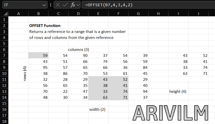
The Excel OFFSET function returns a reference to a range constructed in parts: a starting point, a row and column offset, and a final height and width in rows and columns. OFFSET is handy in formulas that dynamically average or sum “last n values”.
Syntax
The syntax for the OFFSET function in Microsoft Excel is:
=OFFSET( range, rows, columns, [height], [width] )
Parameters or Arguments
range
The starting range from which the offset will be applied.
rows
The number of rows to apply as the offset to the range. This can be a positive or negative number.
columns
The number of columns to apply as the offset to the range. This can be a positive or negative number.
height
Optional. It is the number of rows that you want the returned range to be. If this parameter is omitted, it is assumed to be the height of range.
width
Optional. It is the number of columns that you want the returned range to be. If this parameter is omitted, it is assumed to be the width of range.
The Offset Function is an Array Formula
If the Offset function is used alone (i.e. not supplied directly to another function), and the returned range consists of more than one cell, the Offset function must either be entered as an Array Formula).
To input an array formula, you need to first highlight the range of cells that are to contain the function result. Type your function into the first cell of the range, and press Ctrl+Shift+Enter. This is illustrated in Examples 2 & 3 below. If you are using MS Office 365, you can directly write the formula just like other formulas.
Offset Function Examples
In each of the following Offset function examples, the reference range is highlighted in green and the returned offset range is shown in red.
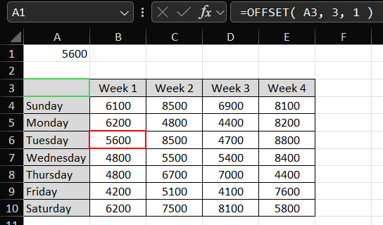
Example 1In the example on the right, the Excel Offset function is used to offset cell A3 by three rows and one column. This returns a reference to cell B6, and so the value of cell B6 is displayed. =OFFSET( A3, 3, 1 ) Note that, in this example:
|  |
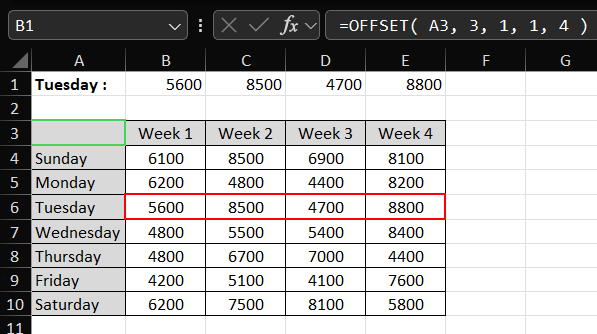
Example 2In the example on the right, the Offset function is used to offset cell A3 by three rows and one column and to return a range that spans one row and four columns. This returns the range, B6-E6. =OFFSET( A3, 3, 1, 1, 4 ) Note that, in this example:
|  |
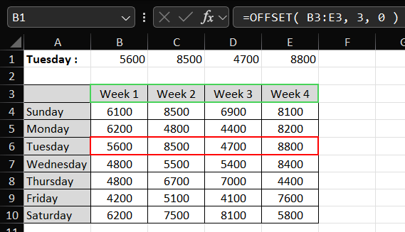
Example 3In the example on the right, the Offset function is used to offset cells B3-E3 by three rows (and zero columns). This returns the range, B6-E6. =OFFSET( B3:E3, 3, 0 ) Note that, in this example:
|  |
Example 4In the example on the right, the Offset function is used to offset cell A3 by one row and one columns. This returns the range B4-B10 (containing the figures for week 1). The returned range is then provided as an argument to the Excel SUM function. As shown in the formula bar, the formula used is: =SUM(OFFSET(A3,1,1,7)) Note that, in this example:
| 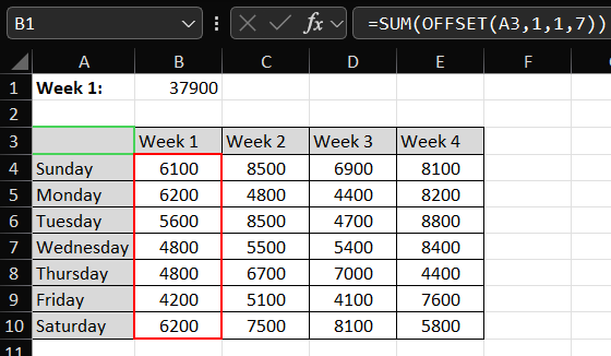 |
Notes
- OFFSET returns a reference to a range that is offset from a starting point in a worksheet. The starting point can be one cell or a range of cells, and the offset is supplied as rows or columns “offset” from the starting point. The height and width arguments are optional and determine the size of the reference that is created.
- OFFSET can be used to build a dynamic named range for charts or pivot tables, to make sure that source data is always up to date.
- OFFSET only returns a reference, no cells are moved.
- Both rows and cols can be supplied as negative numbers to reverse their normal offset direction – negative cols offset to the left, and negative rows offset above.
- OFFSET is a “volatile” formula; it is recalculated whenever there is any change to a worksheet. It can slow down Excel in a complicated worksheet.
- OFFSET will display the #REF! error value if the offset is outside the edge of the worksheet.
- When height or width is omitted, the height and width of reference is used.
- OFFSET can be used with any other function that expects to receive a reference.