SUMIFS is a function to sum cells that meet multiple criteria. SUMIFS can be used to sum values when adjacent cells meet criteria based on dates, numbers, and text. SUMIFS supports logical operators (>,<,<>,=) and wildcards (*,?) for partial matching.
Syntax
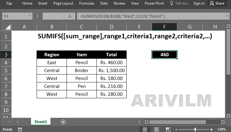
The syntax for the SUMIFS function in Microsoft Excel is:
SUMIFS( sum_range, criteria_range1, criteria1, [criteria_range2, criteria2, ... criteria_range_n, criteria_n] )
Parameters or Arguments
sum_range
The cells to sum.
criteria_range1
The range of cells that you want to apply criteria1 against.
criteria1
It is used to determine which cells to add. criteria1 is applied against criteria_range1.
criteria_range2, … criteria_range_n
Optional. It is the range of cells that you want to apply criteria2, … criteria_n against. There can be up to 127 ranges.
criteria2, … criteria_n
Optional. It is used to determine which cells to add. criteria2 is applied against criteria_range2, criteria3 is applied against criteria_range3, and so on. There can be up to 127 criteria.
Excel Sumifs Function Examples
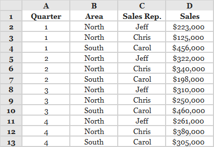
The spreadsheet below shows the quarterly sales figures for 3 sales representatives.
The Sumifs function can be used to find total sales figures for any combination of quarter, area and sales rep.
This is shown in the examples below.
Example 1
To find the sum of sales in the North area during quarter 1:
=SUMIFS( D2:D13, A2:A13, 1, B2:B13, "North" )
which gives the result $348,000.
In this example, the Excel Sumifs function identifies rows where:
– The value in column A is equal to 1
And
– The entry in column B is equal to “North”
and calculates the sum of the corresponding values from column D.
I.e. this formula finds the sum of the values $223,000 and $125,000 (from cells D2 and D3).
Example 2
Again, using the data spreadsheet above, we can also use the Sumifs function to find the total sales for “Jeff”, during quarters 3 and 4:
=SUMIFS( D2:D13, A2:A13, ">2", C2:C13, "Jeff" )
This formula returns the result $571,000.
In this example, the Excel Sumifs function identifies rows where:
– The value in column A is greater than 2
And
– The entry in column C is equal to “Jeff”
and calculates the sum of the corresponding values in column D.
I.e. this formula finds the sum of the values $310,000 and $261,000 (from cells D8 and D11).
Notes
SUMIFS sums cells in a range that match supplied criteria. Unlike the SUMIF function, SUMIFS can apply more than one set of criteria, with more than one range. The first range is the range to be summed. The criteria are supplied in pairs (range/criteria) and only the first pair is required. For each additional criterion, supply an additional range/criteria pair. Up to 127 range/criteria pairs are allowed.
– Each additional range must have the same number of rows and columns as the sum_range.
– Non-numeric criteria must be enclosed in double quotes, but numeric criteria do not need quotes except with operators, i.e. “>32”
– The wildcard characters ? and * can be used in criteria.
– SUMIF and SUMIFS can handle ranges, but not arrays. This means you can’t use other functions like YEAR on the criteria range, since the result is an array. If you need this functionality, use the SUMPRODUCT function.
– The order of arguments is different between the SUMIFS and SUMIF functions. Sum_range is the first argument in SUMIFS, but the third argument in SUMIF.
– The Excel Sumifs function is not case-sensitive. So, for example, the text strings “TEXT” and “text” will be considered to be equal.
– Error #VALUE Occurs if the supplied sum_range and criteria_range arrays do not all have equal length.
1 thought on “Sumifs() Function”