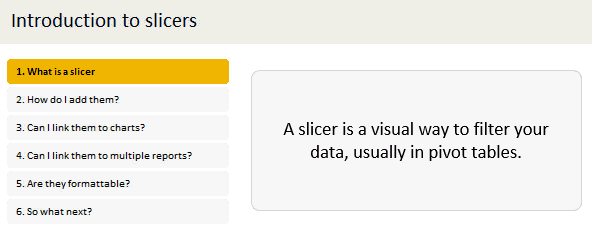
Slicers are visual filters, introduced in Excel 2010. They are a powerful new way to filter pivot table data. Slicers provide buttons that you can click to filter PivotTable data. In addition to quick filtering, slicers also indicate the current filtering state, which makes it easy to understand what exactly is shown in a filtered PivotTable report.
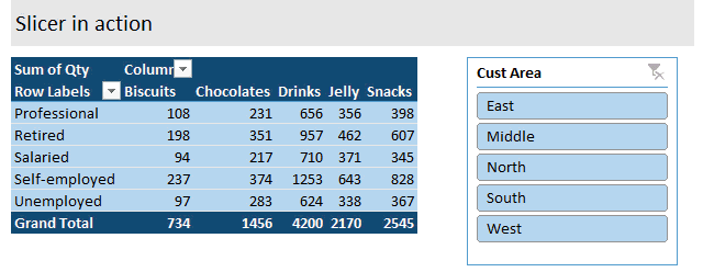
When you select an item, that item is included in the filter and the data for that item will be displayed in the report. For example, when you select East in the Region field, only data that includes East in that field are displayed.
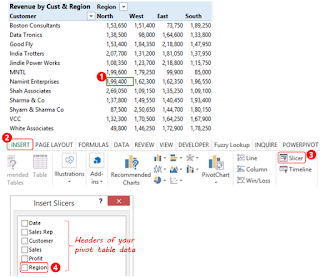
Adding a slicer to a Pivot table
Slicers are typically associated with the PivotTable in which they are created.
- Click on any cell in the pivot table
- Go to the Insert menu and
- Click on Slicer
- In the Insert Slicer Box, choose field/s on which you want the slicer. In our case it will be ‘Region’
- Done! Instantly you’ll get an interactive button displaying all four regions. Clicking any region will filter the pivot table
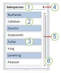
A slicer typically displays the following elements:
- A slicer header indicates the category of the items in the slicer.
- A filtering button that is not selected indicates that the item is not included in the filter.
- A filtering button that is selected indicates that the item is included in the filter.
- A Clear Filter button removes the filter by selecting all items in the slicer.
- A scroll bar enables scrolling when there are more items than are currently visible in the slicer.
- Border moving and resizing controls allow you to change the size and location of the slicer.
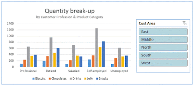
Creating interactive charts with slicers
Since slicers talk to Pivot tables, you can use them to create cool interactive charts in Excel. The basic process is like this:
- Set up a pivot table that gives you the data for your chart.
- Add slicer for interaction on any field (say slicer on customer’s region)
- Create a pivot chart (or even regular chart) from the pivot table data.
- Move slicer next to the chart and format everything to your taste.
- And your interactive chart is ready!