Conditional formatting allows you to automatically apply formatting—such as colors, icons, and data bars—to one or more cells based on the cell value. To do this, you’ll need to create a conditional formatting rule.

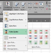
Conditional Formatting Presets

Excel has several predefined styles—or presets—you can use to quickly apply conditional formatting to your data. They are grouped into three categories:

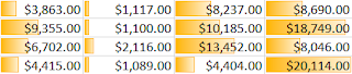
Data Bars are horizontal bars added to each cell, much like a bar graph.

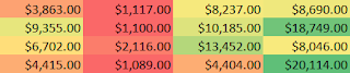
Color Scales change the color of each cell based on its value. Each color scale uses a two- or three-color gradient. For example, in the Green-Yellow-Red color scale, the highest values are green, the average values are yellow, and the lowest values are red.

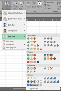
Icon Sets add a specific icon to each cell based on its value.

To Use Preset Conditional Formatting:

1. Select the desired cells for the conditional formatting rule.
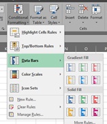
2. Click the Conditional Formatting command. A drop-down menu will appear.
3. Hover the mouse over the desired preset, then choose a preset style from the menu that appears.
4. The conditional formatting will be applied to the selected cells.

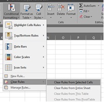
To remove conditional formatting:

1. Click the Conditional Formatting command. A drop-down menu will appear.
2. Hover the mouse over Clear Rules, and choose which rules you want to clear.
3. The conditional formatting will be removed.