Conditional formatting is a fantastic way to quickly visualize data in a spreadsheet. With conditional formatting, you can do things like highlight dates in the next 30 days, flag data entry problems, highlight rows that contain top customers, show duplicates, and more.

Excel ships with a large number of “presets” that make it easy to create new rules without formulas. However, you can also create rules with your own custom formulas. By using your own formula, you take over the condition that triggers a rule, and can apply exactly the logic you need. Formulas give you maximum power and flexibility.

Formula-Based Conditional Formatting

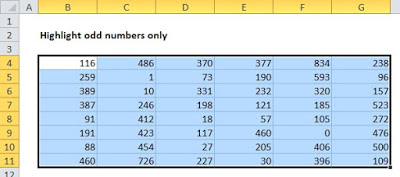
1. Select the cells you want to format.

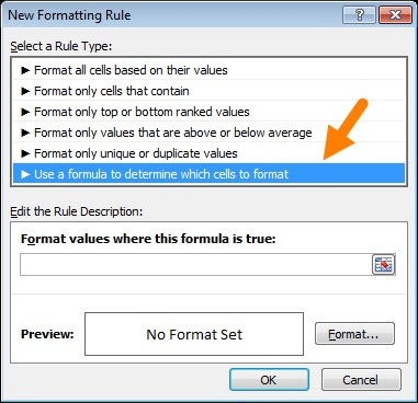
2. Create a conditional formatting rule, and select the Formula option

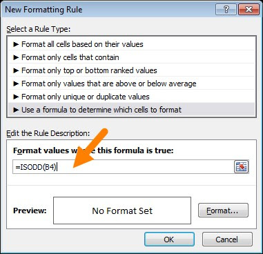
3. Enter a formula that returns TRUE or FALSE.

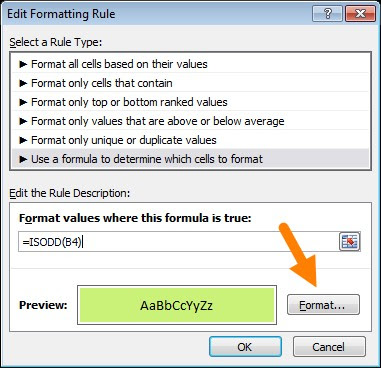
4. Set formatting options and save the rule.

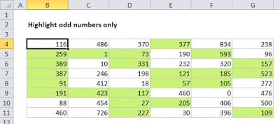
The ISODD function only returns TRUE for odd numbers, triggering the rule:

Reference : https://exceljet.net/conditional-formatting-with-formulas

follow us on http://arivilm.co.in/blog-2/

like us on https://www.facebook.com/Arivilm2501/