Conditional Formatting

Conditional Formatting (CF) is a tool that allows you to apply formats to a cell or range of cells, and have that formatting change depending on the value of the cell or the value of a formula.  When the value of the cell meets the format condition, the format you select is applied to the cell.  If the value of the cell does not meet the format condition, the cell’s default formatting is used.

Formatting vs Conditional Formatting

Formatting, such as currency, alignment, and colour, determines how Excel displays a value. But conditional formatting is more flexible, applying specified formatting only when certain conditions are met.

Create conditional formatting rules

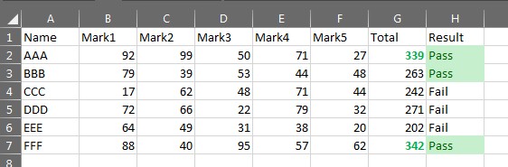
                For Example, let say I want to track the student’s marks and their results.

                In this worksheet, we see the information we want by using conditional formatting, driven by two rules that each contain a formula. First rule in the Total column, formats the marks above 300, which is number and second rule is in the Result column formats the result Pass, which is text.

To create the NUMBER rule:

1. 1. Select cells G2 through G7. Do this by dragging from A2 to A7.

1. 1. Then, click Home > Conditional Formatting > Highlight Cells Rules > Greater Than.

1. 1. In the dialog box, enter 300 and select the format you want.

1. 1. Click OK until the dialog boxes are closed.

1. 1. The formatting is applied to column G.

1. In the same way, we can use Lesser Than and Between options.

To create the TEXT rule:

1. 1. Select cells G2 through G7. Do this by dragging from A2 to A7.

1. 1. Then, click Home > Conditional Formatting > Highlight Cells Rules > Text that contains.

1. 1. In the dialog box, enter Pass and select the format you want.

1. 1. Click OK until the dialog boxes are closed.

1. The formatting is applied to column H.

To be continued..

 follow us on http://arivilm.co.in/blog-2/

like us on https://www.facebook.com/Arivilm2501/