Sort By Cell Formatting:
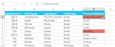
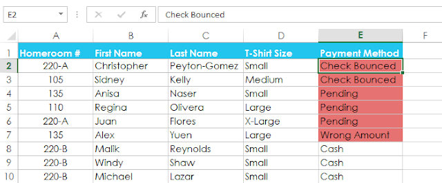
You can also choose to sort your worksheet by formatting rather than cell content. This can be especially helpful if you add color coding to certain cells. In our example below, we’ll sort by cell color to quickly see which T-shirt orders have outstanding payments.
1. Select a cell in the column you want to sort by. In our example, we’ll select cell E2.
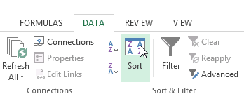
2. Select the Data tab, then click the Sort command.
3. The Sort dialog box will appear. Select the column you want to sort by, then decide whether you’ll sort by Cell Color, Font Color, or Cell Icon from the Sort On field. In our example, we’ll sort by Payment Method(column E) and Cell Color.
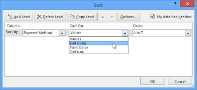
4. Choose a color to sort by from the Order field. In our example, we’ll choose light red.
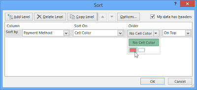
5. Click OK. In our example, the worksheet is now sorted by cell color, with the light red cells on top. This allows us to see which orders still have outstanding payments.
Sort Data by Cell Icon
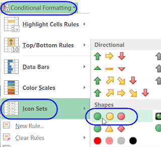
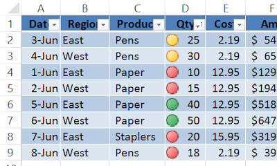
If you add conditional formatting icons to one of the columns, you can also sort by those icons. In the screen shot below, Traffic light icons are being added to the Quantity column.
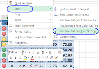
After adding icons, the quickest way to sort by a specific icon is:
- Right-click on a cell that contains the icon you want at the top of the list
- In the pop-up menu, click Sort
- Click Put Selected Cell Icon On Top
The list is sorted, to move all items with the selected icon to the top of the list.
Other items are not sorted, and the items that were moved to the top of the list are left in their original order, within that group.
Sort By Rows To Reorder Columns In Excel
Most of the time when you’re sorting in Excel, you sort based on the values in one or more columns. It’s rare that you sort horizontally, based on the values in a row.
It is possible though, and you can sort in ascending, descending, or custom sort order.
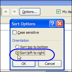
To sort by row, click the Options button in the Sort dialog box. Then, in the Sort Options, select Sort Left to Right.
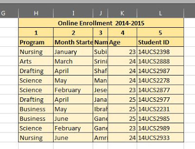
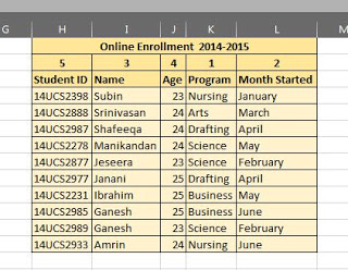
In the data sample used for this series on Excel sort options, the Student ID column has always been first on the left, followed by Name and then usually Age.
In this instance, as shown in the image above, the columns have been reordered so that the Program column is first on the left followed by Month Started,Name, etc.
The following steps were used to change the column order to that seen in the image above:
- Insert a blank row above the row containing the field names
- In this new row, enter the following numbers left to right starting incolumn H: 5, 3, 4, 1, 2
- Highlight the range of H2 to L13
- Click on the Home tab of the ribbon.
- Click on the Sort & Filter icon on the ribbon to open the drop down list.
- Click on Custom Sort in the drop down list to bring up the Sort dialog box
- At the top of the dialog box, click on Options to open the Sort Options dialog box
- In the Orientation section of this second dialog box, click on Sort left to right to sort the order of columns left to right in the worksheet
- Click OK to close this dialog box
- With the change in Orientation, the Column heading in the Sort dialog box changes to Row
- Under the Row heading, choose to sort by Row 2 – the row containing the custom numbers
- The Sort On option is left set to Values
- Under the Sort Order heading, choose Smallest to Largest from the drop down list to sort the numbers in row 2 in ascending order
- Click OK to close the dialog box and sort the columns left to right by the numbers in row 2
- The order of columns should begin with Program followed by Month Started, Name, etc.